Frequency response

Frequency response is the measure of any system's output spectrum in response to an input signal.^[1] In the audible range it is usually referred to in connection with electronic amplifiers, microphones and loudspeakers. Radio spectrum frequency response can refer to measurements of coaxial cables, category cables, video switchers and wireless communications devices. Subsonic frequency response measurements can include earthquakes and electroencephalography (brain waves).

Frequency response requirements differ depending on the application.^[2] In high fidelity audio, an amplifier requires a frequency response of at least 20–20,000 Hz, with a tolerance as tight as ±0.1 dB in the mid-range frequencies around 1000 Hz, however, in telephony, a frequency response of 400–4,000 Hz, with a tolerance of ±1 dB is sufficient for intelligibility of speech.^[2]

Frequency response curves are often used to indicate the accuracy of electronic components or systems.^[1] When a system or component reproduces all desired input signals with no emphasis or attenuation of a particular frequency band, the system or component is said to be "flat", or to have a flat frequency response curve.^[1]

The frequency response is typically characterized by the magnitude of the system's response, measured in decibels (dB), and the phase, measured in radians, versus frequency. The frequency response of a system can be measured by applying a test signal, for example:

applying an impulse to the system and measuring its response (see impulse response)
sweeping a constant-amplitude pure tone through the bandwidth of interest and measuring the output level and phase shift relative to the input
applying a signal with a wide frequency spectrum (for example digitally-generatedmaximum length sequence noise, or analog filtered white noise equivalent, like pink noise), and calculating the impulse response by deconvolution of this input signal and the output signal of the system.

These typical response measurements can be plotted in two ways: by plotting the magnitude and phase measurements to obtain a Bode plot or by plotting the imaginary part of the frequency response against the real part of the frequency response to obtain a Nyquist plot.

Once a frequency response has been measured (e.g., as an impulse response), providing the system is linear and time-invariant, its characteristic can be approximated with arbitrary accuracy by a digital filter. Similarly, if a system is demonstrated to have a poor frequency response, a digital oranalog filter can be applied to the signals prior to their reproduction to compensate for these deficiencies.

Frequency response measurements can be used directly to quantify system performance and design control systems. However, frequency response analysis is not suggested if the system has slow dynamics

The frequency response of an LTI filter may be defined as the spectrum of the output signal divided by the spectrum of the input signal. In this section, we show that the frequency response of any LTI filter is given by its transfer function

evaluated on the unit circle, i.e., $H(e^{j\omega T})$ . We then show that this is the same result we got using sine-wave analysis in Chapter 1.
Beginning with Eq. $\,$ (6.4), we have

$\displaystyle Y(z) = H(z)X(z)$

where X(z) is the z transform of the filter input signal

is the z transform of the output signal

, and

is the filter transfer function.
A basic property of the z transform is that, over the unit circle $z=e^{j\omega T}$ , we find the spectrum [84].^8.1To show this, we set $z=e^{j\omega T}$ in the definition of the ztransform, Eq. $\,$ (6.1), to obtain

$\displaystyle X(e^{j\omega T}) = \sum_{n=-\infty}^\infty x(n) e^{-j\omega T n}$

which may be recognized as the definition of the bilateral discrete time Fourier transform (DTFT) when

is normalized to 1 [59,84]. When

is causal, this definition reduces to the usual (unilateral) DTFT definition:

DTFT $\displaystyle _\omega(x) \isdefs \sum_{n=0}^\infty x(n) e^{-j\omega n} \protect$

(8.1)

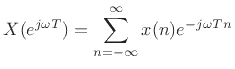
Applying this relation to

gives

$\displaystyle Y(e^{j\omega T}) = H(e^{j\omega T})X(e^{j\omega T}). \protect$

(8.2)

Thus, the spectrum of the filter output is just the input spectrum times the spectrum of the impulse response $H(e^{j\omega T})$ . We have therefore shown the following:

$\textstyle \parbox{0.8\textwidth}{\emph{The frequency response of a linear tim... ...uated on the unit circle in the $z$ plane, \textit{i.e.}, $H(e^{j\omega T})$.}}$

This immediately implies the following:

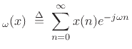
$\textstyle \parbox{0.8\textwidth}{\emph{The frequency response of an LTI filter equals the discrete-time Fourier transform of the impulse response.}}$

We can express this mathematically by writing

$\displaystyle \zbox {H(e^{j\omega T}) = \mbox{{\sc DTFT}}_{\omega T}(h).}$

By Eq. $\,$ (7.2), the frequency response specifies the gain and phase shift applied by the filter at each frequency. Since

, and

are constants, the frequency response $H(e^{j\omega T})$ is only a function of radian frequency $\omega$ . Since $\omega$ is real, the frequency response may be considered a complex-valued function of a real variable. The response at frequency

Hz, for example, is $H(e^{j2\pi f T})$ , where

is the sampling period in seconds. It might be more convenient to define new functions such as $H^\prime(\omega) \isdeftext H(e^{j\omega T})$ and write simply $Y^\prime(\omega) = H^\prime(\omega) X^\prime(\omega)$ instead of having to write $e^{j\omega T}$ so often, but doing so would add a lot of new functions to an already notation-rich scenario. Furthermore, writing $H(e^{j\omega T})$ makes explicit the connection between the transfer function and the frequency response.
Notice that defining the frequency response as a function of $e^{j\omega T}$ places the frequency ``axis'' on the unit circle in the complex

plane, since $\left\vert e^{j\omega T}\right\vert=1$ . As a result, adding multiples of the sampling frequency to $\omega$ corresponds to traversing whole cycles around the unit circle, since

$\displaystyle e^{j(\omega + k 2\pi f_s)T} = e^{j(\omega T + k 2\pi)} = e^{j\omega T},$

whenever

is an integer. Since every discrete-time spectrum repeats in frequency with a ``period'' equal to the sampling rate, we may restrict $\omega T$ to one traversal of the unit circle; a typical choice is $-\pi \leq \omega T < \pi$ [ $\omega T\in[-\pi,\pi)$ ]. For convenience, $\omega T \in[-\pi,\pi]$ is often allowed.
We have seen that the spectrum is a particular slice through the transfer function. It is also possible to go the other way and generalize the spectrum (defined only over the unit circle) to the entire

plane by means of analytic continuation (§D.2). Since analytic continuation is unique (for all filters encountered in practice), we get the same result going either direction.
Because every complex number

can be represented as a magnitude $r=\vert z\vert$ and angle $\theta=\angle z$ , viz., $z=r\exp(j\theta)$ , the frequency response $H(e^{j\omega T})$ may be decomposed into two real-valued functions, the amplitude response $\vert H(e^{j\omega T})\vert$ and the phase response $\angle H(e^{j\omega T})$ . Formally, we may define them as follows:

Frequency Response Ranges

You will often see frequency response quoted as a range between two figures. This is a simple (or perhaps "simplistic") way to see which frequencies a microphone is capable of capturing effectively. For example, a microphone which is said to have a frequency response of 20 Hz to 20 kHz can reproduce all frequencies within this range. Frequencies outside this range will be reproduced to a much lesser extent or not at all.

This specification makes no mention of the response curve, or how successfully the various frequencies will be reproduced. Like many specifications, it should be taken as a guide only.

HENDERSON PARADA

http://en.wikipedia.org/wiki/Frequency_response

https://ccrma.stanford.edu/~jos/fp/Frequency_Response_I.html

http://www.mediacollege.com/audio/microphones/frequency-response.html